How to enable finder to show all hidden files Mac OS X 10.8

Type the following commands in Terminal:

defaults write com.apple.Finder AppleShowAllFiles YES
killall -HUP Finder

The first command sets a hidden preference so the finder shows all files and the second command restarts the Finder so these preferences take effect. The kill all command tells Finder to quit while the -HUP flag asks the program to restart.

The files can be hidden by typing the following into Terminal:

defaults write com.apple.Finder AppleShowAllFiles NO
killall -HUP Finder

If these commands do not work try a lower case F in the word Finder in the following command:

defaults write com.apple.Finder AppleShowAllFiles

Divide and Conquer Inversion Counting Algorithm vs Brute Force

First I will generate a random array of size 100,000 for both algorithms and then proceed with counting the number of inversions in the generated array according to the corresponding algorithm. Here are both algoritms and I will discuss the run times later

1. Divide and Conquer Algorithm
from random import randint


def generate_array():
    length_of_array = 100000
    i = 0
    array = []
    while i < length_of_array:
        array.append(randint(0,length_of_array))
        i += 1

    return array

def sort_count(A,B):
    global inversions
    C=[]
    lenA = len(A)
    lenB = len(B)
    i, j = 0, 0
    while i < lenA and j < lenB:
        if A[i] <= B[j]:
            C.append(A[i])
            i=i+1
        else:
            inversions= inversions +len(A)-i #the maggic happens here
            C.append(B[j])
            j=j+1
    if i == lenA:#A get to the end
        C.extend(B[j:])
    else:
        C.extend(A[i:])
    return C # sends C back to divide_array which send that back to the divide_array
             # which called it as the right variable

def divide_array(L):
    N = len(L)
    if N > 1:
        left = divide_array(L[0:N/2])
        right = divide_array(L[N/2:])
        return sort_count(left,right)
    else:
        return L
inversions = 0
array = generate_array()
sorted_array = divide_array(array)
print inversions


2. Brute Force Algorithm

from random import randint


def generate_array():
    length_of_array = 100000
    i = 0
    array = []
    while i < length_of_array:
        array.append(randint(0,length_of_array))
        i += 1

    
    return array


array = generate_array()
i = 0
inversions = 0 
length = len(array)
while i < length:
    for n in array[i+1:]:
        if n < array[i]:
            inversions = inversions + 1
    i = i+1

print inversions


Analysis of Algorithms

So both of these algorithms can complete the job of counting number of inversions however, the Brute Force Algoritm is considerably slower. 

While Divide and Conquer completed the task in 1.325s the Brute Force Algorithm completed the task in 20m35.371s on the same computer.  This is a huge difference! Which shows the power of the Divide and Conquer Algorithm. 

Divide and Conquer runs on O(n log n) time while Brute Force runs on O(n^2) time. Where n is the length of the array. 

Graphic representation of big-Oh comparison for algorithms

Here's the code for making the above graph

from pylab import *

n = arange(1,100)
f2 = n* (log(n))
f = n**2

fig = figure()
ax = fig.add_subplot(111)

ax.plot(f2)
ax.plot(f)

legend(('Divide and Conquer', 'Brute Force'), 'upper left', shadow=True)

title('Divide and Conquer Inversion Counting Algorithm vs Brute Force') 

xlabel('Size of array (n)')
ylabel('Number of interations')

show()

version control and git

Originally version control was developed for large software projects with many developers.  However, it can be useful for single users also.  A single user could use version control to keep track of history and changes to files including word files which will allow them to revert back to previous versions.  Its also useful way to keep many different versions of code well organized and keep work in sync on multiple computers. 

So how does version control work?

The system keeps track of differences from one version to the next by making a changeset which is a collection of differences from one commit.  Then the System can go back and reconstruct any version. Git is a distributed version control system (DVCS) that I will talk about here.

So what is a distributed version control system?  Its a version control system where every person has the complete history of the entire project.  DVCS requires no connection to a central repository, and commits are very fast which allows commits to be much more frequent. Also you can commit changes, revert to earlier versions, and examine history all without being connected to the server and without affecting anyone else's work. Also it isn't a problem if the server dies since every clone has a full history.  Once a developer has made one or more local commits, they can push those changes to another repository or other developer can pull them.  Most projects have a central repository but this is not necessary.  Use this link for branching diagrams.

Changeset all stored in one .git subdirectory in a top directory.  This will be a hidden file since it starts with a  dot.  Its best not to mess with this file however you can see this file in Unix with the ls -a command.

To make a clone use:

git clone (web address of  bitbucket) (name of what you would like to call the file)

git clone will make a complete copy of the repository at the particular directory you have navigated to in terminal.

To make a new git repository:
steps make a directory then Initialized git repository
    mkdir name of directory
    git init

Here is a list of useful git commands:

git add (file name) - adds file to git repository
git add -u - adds anything it the current directory which is already under version control (then do a git commit)
git clone - makes a complete copy of the repository at a particular directory you navigated to in terminal
git checkout (name of commit) - converts everything in repository back to that commit
git checkout (name of commit) -- (name of file to revert back) - converts just that file back to the commit
git checkout HEAD - gits you the most recent commit
git commit - commits to your clone's .git directory -m "string describing commit"
git commit -m "first version of script"
git fetch - pulls changesets from another clone by default: the one you cloned from
git init - Initialize git repository
git ls-files . - tells which files in this directory are under version control currently
git log - Shows most recent commits you did
git merge - applies changesets to your working copy
git pull - updating repository (navigate to the repository on your machine and perform git pull)
git push - sends your recent changesets to another clone by default: the one you clone from
git status - outputs all untracked files
git status | more - shows page by page untracked files
git status . - shows files to be committed in the directory you are in
  Protocol to remove untracked files that you never put in the repository such as .pyc files
   create a special file called .gitignore
    example: $ vi directoryname/.gitignore
   then add the types of files you would like to ignore
    example: *.pyc (ignore any .pyc file)

github vs bitbucket

bitbucket is private and github is public
git was developed for the open source software for the developing the linux kernal
many repository for scientific computing projects use github for example IPython, NumPy, Scipy, and matplotlib








 

A simple introduction to MapReduce

I've grown extremely fond of the MapReduce programming model for processing large sets of data in parallel.

So what is MapReduce?

Well besides being the most wonderful model I've come across so far, it is a program that comprises of a Map() function and a Reduce() function. The Mapper filters and sorts and sends key value pairs to a shuffler and sorter. The shuffler and sorter pairs common keys together and then sends it to the Reducer that summaries the data.

MapReduce Via Cooking

Lets start by making my favorite South Indian Chutney; Chettinad Tomato Chutney.  Please note that the recipe below is just a fragment of the entire recipe.  The picture and full recipe is locate at this link if you would like to try it.



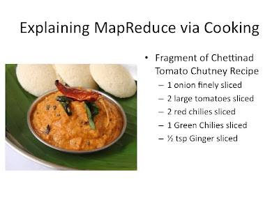
First we would have to slice all the veggies.  As shown below.  This is similar to the mapper function in MapReduce.  The human slicer will throw out all bad veggies and slice all fresh veggies.  The key would be the veggie name and the value would be individual slices.



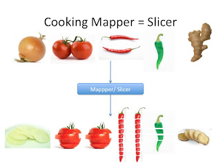
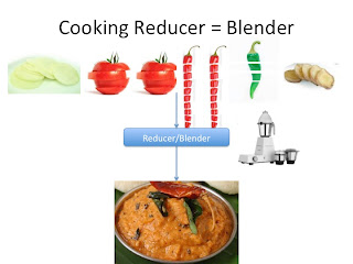
This would be sent to the Shuffler and sorter but we will come back to that.  Now just imagine it is sent directly to the Reducer or Blender.  The blender will mush everything into one tomato chutney dish.  Looks good right?



Now imagine you own a South Indian Restaurant. This restaurant is extremely successful and your famous Chettinad Tomato Chutney is a top seller. Every day you sell at least 150 orders of it.

How would you accomplish this task?

First you will need a large supply of onions, tomatoes, red chilies, green chilies, and ginger
Next you will need to hire a bunch of human slicers
Then you will have to buy many blenders
You will also have to Shuffle and sort sliced similar veggies together from different slicers
Then blend appropriate quantities of each veggie together.

This is MapReduce! Processing a lot of things in parallel.

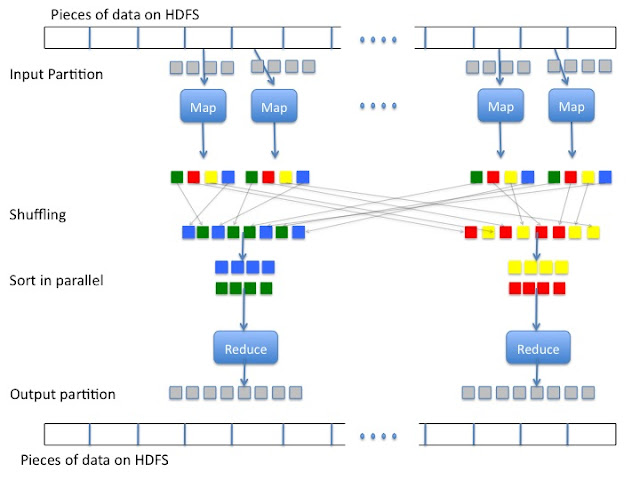
Below you will find an outline of Hadoop and MapReduce.  Hadoop adds to MapReduce a file saving system called Hadoop Distributed File System (HDFS).  I will not talk about HDFS any further here.  The data is stored on HDFS and then partitioned into smaller pieces and sent to the map functions on multiple cores or computers. Map sends key value pairs to the shuffler.  The shuffler will send specific keys to a specific sorter.  The sorter will pair up all keys and append all values to the same key and send it to the reducer where the data is combined together and summarized.  The data is then stored on HDFS.   

Python NumPy Extension

NumPy extension is an open source python extension for use in multi-dimensional arrays and matrices. Numpy also includes a large library of high-level mathematical functions to operate on these arrays. Since python is an interpreted language it will often run slower than compiled programming languages and NumPy was written to address this problem providing multidimensional arrays and functions and operators that operate efficiently on arrays. In NumPy any algorithm that can be expressed primarily as operations on arrays and matrices can run almost as quickly as the equivalent C code because under the hood it calls complied C code.

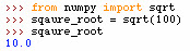
NumPy square root




NumPy array class vs python list

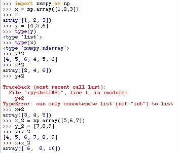
The numpy array is very useful for performing mathematical operations across many numbers. Below you can see that the type list operates very differently than the type numpy.array. Below y is a list and x is a numpy array. Multiplication of lists just repeats the list and addition just concatenates the two lists. However, with the NumPy array component-wise operations are applied.



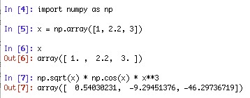
Unlike lists, all elements of a np.array have to be of the same type. On line 5 below np.array was entered as 1(type int), 2.2(type float), and 3(type int). However, on line 6 it was printed out and you can see all values were converted to type float.  Then on line 7 a more complicated component-wise operation was applied to x.



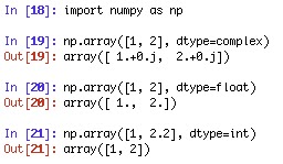
The type of the array can be specified by dtype. Here is a good link for more information on numpy dtype. Below on line 19 the dtype is converted to complex.  Then float and int types are used on line 20 and 21 respectively.




Matrices
Matrices are made by adding lists of lists. Below on line 35 is an example of a 3 by 2 matrix. Then the shape of the matrix is revealed on line 37. On line 38 the matrix is transposed. Then matrix multiplication is accomplished on line 40.



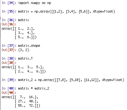
Below is an example of dot product.



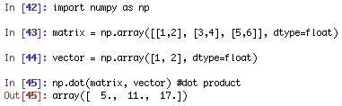
NumPy has another class called matrix which works similar to matlab. However, I like uses nested lists and NumPy array class better. If you would like to use the NumPy matrix class go to this link for more information.

reshape



flatten


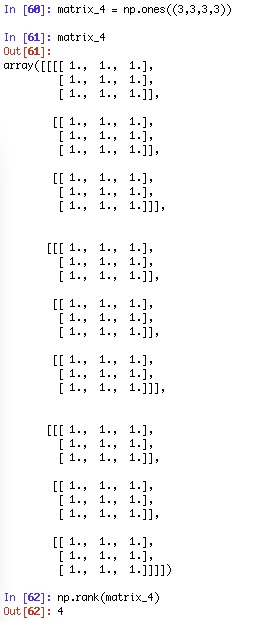
Rank





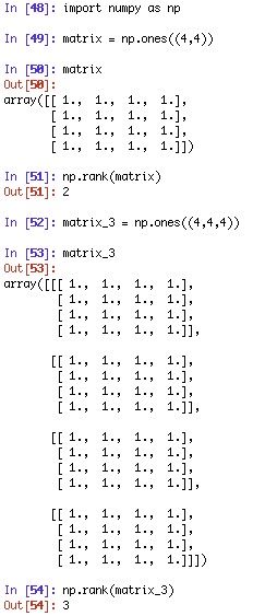
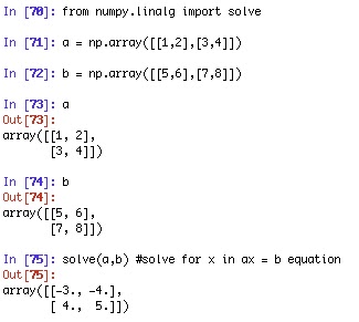
Linear algebra

How to solve for x in ax = b equation



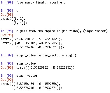
Eigenvalue



numpy not a number

not a number (NaN) value is a special numerical value. NaN represents an undefined or
unrepresentable value mostly in floating-point calculations. Here is an example for a use
of NaN:

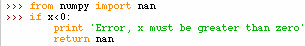
  While writing a square root calculator a return of NaN can be used for ensuring the precondition
  of x is greater than zero. This is how it could be implemented:



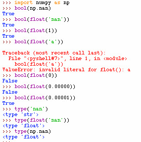
A little more experimenting on numpy nan and python nan concludes that both nans are floating point numbers.  Also  'nan' is of type str but float('nan') is type float.  However, as expected float('a') can not be converted to a float.  From the experiment below you can also see that all floating point numbers return true when you convert to bool type except 0.0.  



For more information visit NaN on Wikipedia

Python tutorial Part 2 time and making folders

The python time module is very useful for finding current time. Below you will find a few examples of the module in use and how to extract year, month, day, hour, minute, second, and microsecond.

To find elapsed time used the the code below.

To make a folder with the current date import sys, os, and datetime.  Use strftime to get the Year with century as a decimal number, get the month as a decimal number, and the day of the month as a decimal number.  Then test to see if the folder already exists and if not make the folder.  Below you will see the folder which was made by the script to the right of it.

Python tutorial Part 1 variables int, float, str, and simple math

Variables refer to memory addresses that store values.  This means all variables are stored in memory.  Therefore for big data applications you will have to keep this in mind.  You can find out the maximum size of lists, strings, and dicts on your system by the code below:

How to Assign integers to variables and subtraction:

The equal sign (=) is used to assign variables in python.  The negative sign (-) is used for subtraction and type() is used to get the type of the variable.  The type of is int in the case below. For example:

How to Assign floating point numbers to variables and addition:

The positive sign (+) is used for addition

Examples of adding and subtracting float and int:

Division of int:

Floating point division uses (/) sign.  This type of division divides left hand operand by right hand operand and returns a floating point number.   Floor Division uses (//) sign.  This type of division is returns only the whole int part of division without any rounding. The modulus (%) operand returns the remainder. 

Division of float:

Division of float returns only type float and everything else is the same as above.

 



Multiply int and float:

The multiply operand is (*).   If the type is only int it returns int.  If either type is float it returns a float.

Exponent of int and float:

The exponent operand is ( **).  If the type is only int it returns int.  If either type is float it returns a float.

How to assign strings and concatenate strings:

To assign variables to strings inclose strings with (' ') or (" ").  As you can see below strings can be concatenated by the plus sign (+) and if you need a space between the words it needs to be added in.  The type of strings is str.

Variable name guide lines:

For python style use lower_case_with_underscores for variable names.  The words are separated by underscores to improve readability.

Variable names can not start with a number

 

How does Speed Congenics work

I operate a speed congenics core facility and I will explain what this is in this post.  Since I'm in the process of automating a lot of mundane tasks associated with this facility and I'm going to share the code on this blog.

Lets talk about congenics first.

In genetics a congenic mouse is a mouse that differs only at one locus in the genome.  This difference is normally introduced by a molecular genetic technique.  Such molecular genetic techniques can include a knock-in, knock-out, or transgene.
 
    Knock-in - a targeted site of insertion into a particular locus in the mouse genome of a protein coding cDNA sequence
 Knock-out - a targeted deletion of a particular gene in the mouse
 transgene - a random site of insertion of a protein coding cDNA sequence

Inbred mouse strains are mice which are the same at every locus.  A very common inbred mouse strain is the C57BL/6 (I will call this mouse B6) mouse.  This inbred mouse strain is favored because it was the first mouse that was fully sequenced.  Therefore just by inertia it became the most widely used and studied inbred mouse strain.  

However, every genetically modified mouse is not made on the B6 background and not every researcher uses the B6 inbred mouse.  Therefore via breeding the mouse needs to be transfered onto the B6 background or the background of the researchers choice.

Now keep in mind the Binary search algorithm.

Example: a guess the number game between 0 and 100.  Use binary search.              

Each time we guess, we guess the number right in the middle. 

                                                            100                            feedback                    #of Guesses

                                                         Guess 50                           Less                             1

                                                         Guess 25                           Less                             2

                                                         Guess 12                           greater                          3

                                                         Guess 18                           greater                          4

                                                         Guess 21                           greater                          5                   

                                                         Guess 23                           Less                              6  

                                                         Guess 22                           Correct                         7 

           

However, in the case of speed congenics our guess number is always 100 because we are trying to transfer from 0% B6 (I will use B6 is the example recipient background) to ~99% B6.  Also the speediest way to get this accomplished is fairly close to  the same as the worst case scenario of binary search.

Speed Congenics reduces time of backcrossing by choosing the best mouse of each generation.  Traditional backcrossing can take 12 generations (3-4 years).  When the best mouse is chosen from each generation it can take 5-6 generations (1.5 - 2 years). 

To make everything as efficient as possible a backcross protocol is followed that maximizes number of mice and cleans the sex chromosomes very quickly.  Highest percent B6 mice are chosen by microsatellite Analysis that covers a full genome every 10 cM. The primers are fluorescently labeled and multiplexed to reduce time.  The pictures below is a backcross of one one from the CBA background to the B6 background. These are actual results for each generation.

So what are microsatellites?  Microsatellites are short tandem repeats of DNA.  Here is an example:GCT AC AC AC AC CA AC AA AC GT  This example has Di-nucleotide (AC) and tri-nucleotide (CAA) repeats.  Microsatellites are useful for speed congenics because they are polymorphic between mouse strains.  Here's an example of peaks seen in Genemapper software.  You can see here that each of three different mouse strains have a different size for this particular microsatellite marker.

Here is an example of a heterozygous marker vs a homozygous marker. The analysis of process if very time consuming.  Some automatic calling via the genemapper software is completed but it take a lot of manual time to transfer the data into a "picture" so the customers can easily understand the data. I'm still thinking about the best way to automate this.

Here is a little outline of the entire process.  I will be writing and posting programs for the Design of panel  and Analysis steps of this process.

 

Mixed starting strain to one ending strain

I run a small mouse speed congenics facility.   I use microsatellite analysis to find the highest percent mouse for each generation. Panels of multiplexed primers are used to distinguish between one inbred mouse strain and the other.  The panels include primers that are polymorphic between the two inbred mouse strains. Each panel has been tested for multiplexing and includes up to 3 fluorescencly labeled primer sets in each well.  The entire system is set up to run in a 96 well format.     

I get many different types of projects and my panels are set up to go from one starting inbred mouse strain to one ending inbred mouse strain.  The function will returns a file containing a multiplexed plate or plates that needs to run that includes all the primers missing in the first plate but present in the second plate.

Example use of this function:

   |       A customer comes to start a speed congenics project however the

   |       starting strain of the project is mixed.  For example the starting

   |       strain is 129 and C3H combined.  The customer wants to cross this

   |       mouse onto the B6 background.  Therefore the best approach would be

   |       to run a full 129XB6 screen and then run the primers that are present

   |       in the B6XC3H screen and not in the 129XB6 screen.

       

here's the code

How big is google's index?

Since Google has stopped exposing the size of their indexed web documents on their homepage, it seems that different web users have been performing searches to try and figure out Google’s size.

Here is my method for figuring out how big google's index is.  

A. Find out how what are the top ten languages on the internet.

     according to: http://www.internetworldstats.com/stats7.htm

     1. English 536.6 million users

     2. Chinese 444.9 million users

     3. Spanish 153.3 million users

     4. Japanese 99.1 million users

     5. Portuguese 82.5 million users

     6. German 75.2 million users

     7. Arabic 65.4 million users

     8. French 59.8 million users

     9. Russian 59.7 million users

     10. Korean 39.4 million users

     11. all the rest of the languages 350.6 million users

B.  Use the most common word of each language as search term

    1. search the word in resulted in 25,270,000,000

    2. searched 啊 2,320,000,000

    3. searched a partir de 1,110,000,000  

    4. searched for で 6,080,000,000

    5. Did not know how to search for portuguese since the words over lapped spanish

    6. searched for das 3,680,000,000

    7. search for في  2,250,000,000 
    8. searched for Le 8,140,000,000
    9. searched for и  4,500,000,000
    10. searched for 에  2,420,000,000
C. add them all up 55,770,000,000
     

Two different ways to translate mRNA to Protein

from Bio.Seq import Seq
from Bio.Alphabet import IUPAC


def translate(mRNA):
    '''(str) -> str

    input is mRNA string and it returns a the corresponding protein string.

    >>>translate('AUGGCCAUGGCGCCCAGAACUGAGAUCAAUAGUACCCGUAUUAACGGGUGA')
    MAMPRTEINSTRING

    Precondition: mRNA has to be Uppercase and include only GAUC
   
    '''
    #IUPAC.unambiguous_rna includes only Uppercase and GAUC
    messenger_rna = Seq(mRNA, IUPAC.unambiguous_rna)
    #translate using a dict already stored in the method
    protein = messenger_rna.translate()

    print protein

--------------------------------------------

def translate_2(mRNA):
    '''(str) -> str

    input is mRNA string and it returns a the corresponding protein string.

    >>>translate('AUGGCCAUGGCGCCCAGAACUGAGAUCAAUAGUACCCGUAUUAACGGGUGA')
    MAMPRTEINSTRING
   
    '''
    #this string will be used to make a dict
    translation_table = '''UUU F      CUU L      AUU I      GUU V
    UUC F      CUC L      AUC I      GUC V
    UUA L      CUA L      AUA I      GUA V
    UUG L      CUG L      AUG M      GUG V
    UCU S      CCU P      ACU T      GCU A
    UCC S      CCC P      ACC T      GCC A
    UCA S      CCA P      ACA T      GCA A
    UCG S      CCG P      ACG T      GCG A
    UAU Y      CAU H      AAU N      GAU D
    UAC Y      CAC H      AAC N      GAC D
    UAA Stop   CAA Q      AAA K      GAA E
    UAG Stop   CAG Q      AAG K      GAG E
    UGU C      CGU R      AGU S      GGU G
    UGC C      CGC R      AGC S      GGC G
    UGA Stop   CGA R      AGA R      GGA G
    UGG W      CGG R      AGG R      GGG G'''

    #Make a list of the above string and remove all spaces or '/n
    translation_list =  translation_table.split()
    #Make dictionary from list
    translation_dict = dict(zip(translation_list[0::2], translation_list[1::2]))

    #Accumulator variable
    protein = ''
    for aa in range(0, len(mRNA)-3, 3):
        protein += translation_dict[mRNA[aa:aa+3]]

    print protein

Installing biopython on Mac OS X 10.5 and Mac OS X 10.8

Installing on Mac OS X 10.5

1. Install XCode
 - https://connect.apple.com/cgi-bin/WebObjects/MemberSite.woa/wa/getSoftware?bundleID=20414 from apple
 - Just use default install 

2.  Install NumPy
 - download http://sourceforge.net/projects/numpy/files/
 - double click on the file and it will unzip
 - I then placed the unzipped file on the desktop(shorter directory address)
 - then open terminal
 - navigate to the file
  - example
   cd /Users/computername/Desktop/numpy-1.7.0
 - then type in terminal python setup.py build (note this takes a little while to complete and as some  points it looks like to stalled.  Just wait.)
 - then type into terminal sudo python setup.py install

3. Install biopython
 - download source zip file from http://biopython.org/wiki/Download
 - double click on it and it will unzip
 - I then placed the unzipped file on the desktop(shorter directory address)
 - then open terminal
 - navigate to the file
 - type python setup.py build
 - python setup.py test
 - sudo python setup.py install

4. go to idle and test if you installed everything

>>> import numpy
>>> print numpy.__version__
1.7.0

>>> import Bio

>>> print Bio.__version__
1.61 

Installing on Mac OS X 10.8

1. Install XCode.
  - Download XCode from the Mac App Store and install

2. Install XCode the command line tools
  - Open XCode
  - Go to XCode on toolbar -> preferences -> Downloads -> click on install Command Line Tools
   - Command Line Tools are already installed on my computer therefore it says update

3. Install MacPorts
  - Download Mountain Lion MacPorts "pkg" installer

4.  Install NumPy
 - download http://sourceforge.net/projects/numpy/files/
 - double click on the file and it will unzip

 - I then placed the unzipped file on the desktop(shorter directory address)
 - then open terminal
 - navigate to the file
  - example
   cd /Users/computername/Desktop/numpy-1.7.0
 - then type in terminal python setup.py build (note this takes a little while to complete and as some  points it looks like to stalled.  Just wait.)
 - then type into terminal sudo python setup.py install

5. Install biopython
 - download source zip file from http://biopython.org/wiki/Download
 - double click on it and it will unzip
 - I then placed the unzipped file on the desktop(shorter directory address)
 - then open terminal
 - navigate to the file
 - type python setup.py build
 - python setup.py test
 - sudo python setup.py install

6. go to idle and test if you installed everything

>>> import numpy
>>> print numpy.__version__
1.7.0

>>> import Bio

>>> print Bio.__version__
1.61 

Translate DNA to RNA

def dna_to_rna(dna):
    '''(str) -> str

    Replace every T with a U
    
    >>>dna_to_rna('GTACTT')
    GUACUU

    >>>dna_to_rna('GGGGTTTTTCCCCTTTTTATCTGT')
    'GGGGUUUUUCCCCUUUUUAUCUGU'

    >>>dna_to_rna('TTTTTTTT')
    UUUUUUUU

    >>>dna_to_rna('TTAA')
    UUAA
    '''

    i = 0
    accum_s = ' '
    last_t_index = 0
    while i < len(dna):
        if dna[i] == 'T':
            accum_s = accum_s + dna[last_t_index: i] + 'U'
            last_t_index = i +1
        i = i + 1
    if last_t_index != len(dna):
        accum_s = accum_s + dna[last_t_index:len(dna)]
    print accum_s

Add Packages for importing to python

Add the package directly to a directory already in the sys.path
1. Find the directory /Library/Frameworks/Python.framework/Versions/3.2/lib/python3.2/site-packages

2. If this folder is hinden in finder and you would like to see it just follow these steps:
    a.  open find
    b.  press shift-Command-G
    c. this brings up a ''go to folder" dialog
    d. Type in the name of the directory.
    e. Then I just dragged this folder under Favorites on the left menu bar.


3.  Now that I just created a test program called hello_world.py
4. I placed hello_world.py in /Library/Frameworks/Python.framework/Versions/3.2/lib/python3.2/site-packages

    def add(A, B):
       print (A + B)


5. opened idle and typed the below commands.

>>> import hello_world
>>> hello_world.add(5,3)
8
>>>

6. now I can import hello_world.add() any time.  I'm now on my way to install any modules.

Add a directory to sys.path

Convert a CPM .txt file to a new DPM .txt file

This little function will take a file full of CPM values and convert it to DPM values in a new file.  This is very useful for wipe tests.

example data:
wipe test 3/15/13 results in cpm
number 24 is blank
   
    1 = 29
    2 = 34
    3 = 31
    4 = 24
    5 = 34
    6 = 27
    7 = 26
    8 = 35
    9 = 25
    10 = 31
    11 = 31
    12 = 25
    13 = 23
    14 = 34
    15 = 37
    16 = 32
    17 = 28
    18 = 35
    19 = 29
    20 = 29
    21 = 35
    22 = 27
    23 = 31
    24 = 32

Example output data:
converted DPM values

1 = 0
2 = 2.86
3 = 0
4 = 0
5 = 2.86
6 = 0
7 = 0
8 = 4.29
9 = 0
10 = 0
11 = 0
12 = 0
13 = 0
14 = 2.86
15 = 7.15
16 = 0
17 = 0
18 = 4.29
19 = 0
20 = 0
21 = 4.29
22 = 0
23 = 0
24 = 0


def CPM_to_DPM(CPM_file, DPM_file):
    # open the files
    CPM_file = open(CPM_file, 'r') # read CPM_file
    DPM_file = open(DPM_file, 'w') # write DPM_file

    # Skip over header
    line = CPM_file.readline()
    while line != '\n':
        line = CPM_file.readline()
  
    # slice out  '1 = ' and record the rest as an int in cpm_data variable
    line = CPM_file.readline()
    cpm_data = [] # accumaltor variable
    while line != "":

        cpm = line[line.rfind(' ') + 1:]
        cpm_data.append(int(cpm))
        line = CPM_file.readline()

    #set last int in array to background
    background = cpm_data[-1]
   
    #go over list if bigger than background perform cpm to dpm equation. if smaller value = 0
    dpm_value = []
    for i in cpm_data:
        if i > background:
            dpm_values = (i - background)*1.43
            dpm_values = round(dpm_values, 2)
            dpm_value.append(dpm_values)
        else:
            dpm_value.append(0)
   
     # write a header on DPM file
    DPM_file.write('converted DPM values')
    DPM_file.write('\n')
    DPM_file.write('\n')
   
    #write dpm_value to DPM file with increasing number for each line
    sample_num = 0
   
    for i in dpm_value:
        sample_num = sample_num + 1
        DPM_file.write(str(sample_num) + ' = ' + str(i))
        DPM_file.write('\n')
       
    # close files
    CPM_file.close()
    DPM_file.close()


    #print done so the user knows to go to look at their dpm file
    print ('done')

pong with CodeSkulptor

I started taking a course on coursera.  The course is called An introduction to Interactive Programming in Python.  It teaches event driven programming.  Until this course I've only been using linear programming.  While  event driven programming is not the answer to every project it is awesome for games which is a huge interest of mine.  At the end of week 4 the mini project was pong.  I changed the code a little as you can see it looks like a little hockey rink. The game only works on at codeskulptor.  Maybe later I will try to use tkinker.  Here's the code! Just copy and paste it into CodeSkulptor!

Implementation of classic arcade game Pong!

 

here's the code

python

This function written is python shortens the string of a .txt file on every other line and makes a copy in a new file.  This is very useful in bioinformatics.  My problem was I had a Phred file from Illumina sequencing where both ends of the sequence was N.  If I map this using bowtie and allow two low quality reads per sequence a lot of the data would be thrown out. 

Simple example:
    +
    Shorten
    Keep
    Shorten
    Keep

    ----------------
Example output
    +
    horte
    Keep
    horte
    Keep
------------------
def every_other_line_shorten(starting_file, ending_file):
# open the files
    from_file = open(starting_file, 'r') # read from file

    to_file = open(ending_file, 'w') # write to_file

    line = from_file.readline()
    while line != "":
   
        # keeps line
        to_file.write(line)
        line = from_file.readline()
       
       # cuts line
         to_file.write(line[1:-2] + '\n')
        line = from_file.readline()

    print('done')
   
    to_file.close()
    from_file.close()